Data Blog Menu

• Home
• About
• Posts
• Contact

Weather analysis in Greece

Analysis and Visualisation of weather conditions in Greece

Posted by Christodoulos Santorinaios on July 24, 2022

Exploring the Weather in Athens

In this assignment we explore the weather in Athens over a period of more than 50 years. This assignment was done as a project for the Practical Data Science course taught by Mr. Panos Louridas at the Athens University of Economics and Business.

---

Questions

Q1: Obtain the Data

We work with data covering the period from 1955 to 2020. The data are obtained from two sources:

• Data downloaded from the National Oceanic and Atmospheric Administration's National Centers for Environmental Information (https://www.ncdc.noaa.gov/cdo-web/) and in particular https://www.ncdc.noaa.gov/cdo-web/search.

• As we are focusing on Athens, we use the data from the Hellinikon weather station and we concentrate on the average daily temperature and precipitation.

• We firstly explore the completeness of the data. What data are missing?

• To fill in any missing data we will will use an alternative dataset available from https://data.hellenicdataservice.gr/dataset/66e1c19a-7b0e-456f-b465-b301a1130e3f; this dataset covers only the period from 2010-2019.

---

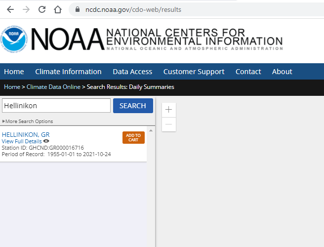
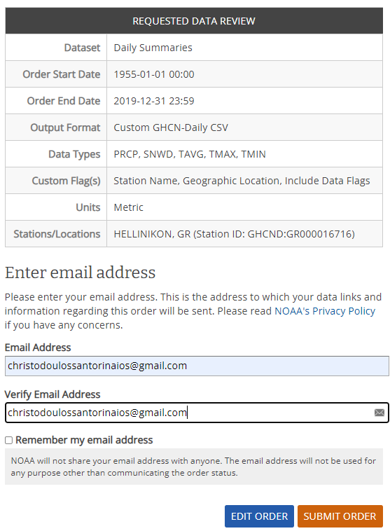
To download the data from the National Oceanic and Atmospheric Administration's National Centers for Environmental Information we follow the steps below.

1. We start by navigating to the https://www.ncdc.noaa.gov/cdo-web/search and inputting the required fields for our search as seen below. Here we fill the fields with values:
   • Dataset: Daily Summaries
   • Date Range: 1955-01-01 to 2019-12-31
   • Search for: Stations
   • Search Term: Hellinikon

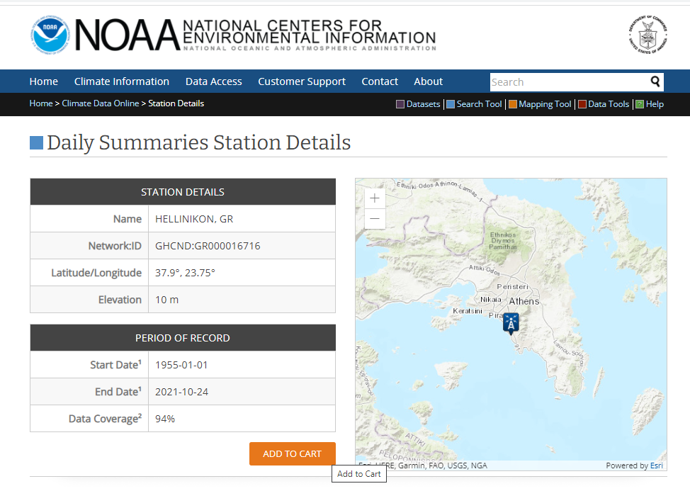
1. In the page that loads, we select the Hellinikon station in the upper left side.
   
   
2. Next we add the dataset to the cart
   
   
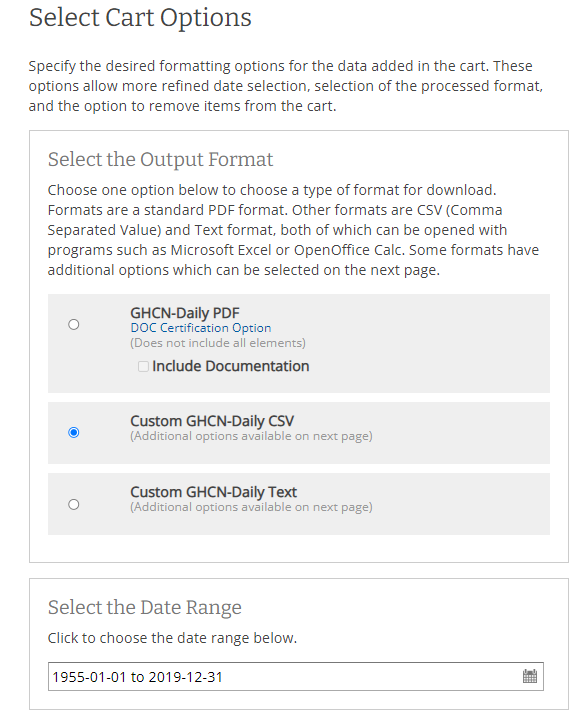
3. In the cart options we select csv format and the date range for which we want to collect the data
   
   
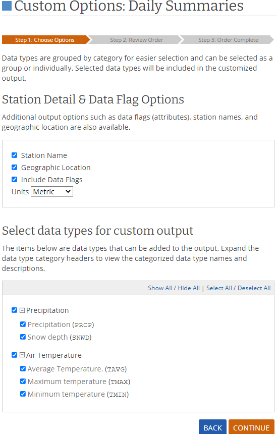
4. At the custom options we select the fields we want to have in our dataset and the units of our data (metric). For our case we should only select data about temperature and precipitation, but I select all the fields just to be safe
   
   
5. In the page that loads we can confirm our selections and place our order by inputting a valid email address. It's safe to input a personal or business email address here as NOAA will use the email address for the sole purpose of communicating the order status to us.
   
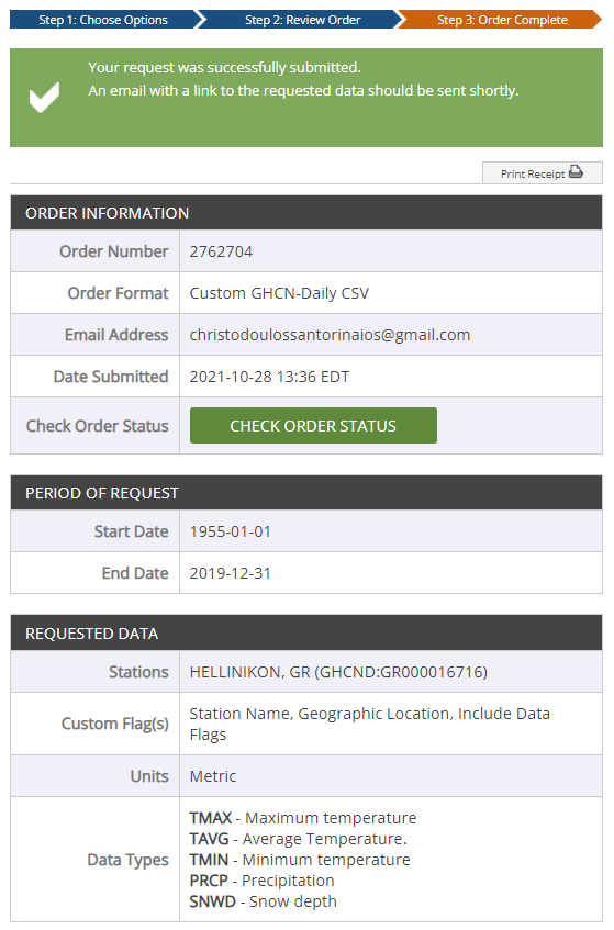
6. After submitting the request we are informed that the order is complete and get various information about the dataset. After a couple of minutes we receive a link to our email with the dataset or we can check order status and the download link will be there.
   

We have two options here. We can use the download link to connect to the csv online (although it expires after 30 days) or we can download and work with dataset locally. I chose the second option.

Now that we have the data, let's import the libraries we are going to use in our analysis.

#import required libraries
%matplotlib inline
import pandas as pd
import matplotlib.pyplot as plt
import matplotlib
import seaborn as sns
matplotlib.rcParams['figure.dpi'] = 300

We read the data and it's important here to use the parse_dates argument to get the dates as datetime64 objects.

# read csv as dataframe parsing dates

df = pd.read_csv('noaa.csv', parse_dates=['DATE'])

Let's have a look on our data, descriptive statistics, missing values, etc. to get a first understanding of what's going on.

df.shape

(22885, 16)

df.sample(10)

	STATION	NAME	LATITUDE	LONGITUDE	ELEVATION	DATE	PRCP	PRCP_ATTRIBUTES	SNWD	SNWD_ATTRIBUTES	TAVG	TAVG_ATTRIBUTES	TMAX	TMAX_ATTRIBUTES	TMIN	TMIN_ATTRIBUTES
8359	GR000016716	HELLINIKON, GR	37.9	23.75	10.0	1977-11-20	15.9	,,E	NaN	NaN	15.9	H,,S	18.6	,,E	12.1	,,E
2476	GR000016716	HELLINIKON, GR	37.9	23.75	10.0	1961-10-12	0.0	,,E	NaN	NaN	16.1	H,,S	18.6	,,E	14.3	,,E
17224	GR000016716	HELLINIKON, GR	37.9	23.75	10.0	2002-02-27	0.0	,,E	NaN	NaN	12.9	H,,S	17.0	,,E	9.2	,,E
8178	GR000016716	HELLINIKON, GR	37.9	23.75	10.0	1977-05-23	0.0	,,E	NaN	NaN	23.9	H,,S	27.6	,,E	19.8	,,E
3632	GR000016716	HELLINIKON, GR	37.9	23.75	10.0	1964-12-11	0.0	,,E	NaN	NaN	11.8	H,,S	12.0	,,E	10.6	,,E
9457	GR000016716	HELLINIKON, GR	37.9	23.75	10.0	1980-11-22	0.0	,,E	NaN	NaN	10.7	H,,S	16.0	,,E	5.4	,,E
21512	GR000016716	HELLINIKON, GR	37.9	23.75	10.0	2016-03-05	0.8	,,S	NaN	NaN	13.3	H,,S	16.8	,,S	8.6	,,S
3238	GR000016716	HELLINIKON, GR	37.9	23.75	10.0	1963-11-13	0.0	,,E	NaN	NaN	19.9	H,,S	23.6	,,E	16.2	,,E
14962	GR000016716	HELLINIKON, GR	37.9	23.75	10.0	1995-12-19	4.0	,,E	NaN	NaN	13.6	H,,S	15.6	,,E	9.2	,,E
3785	GR000016716	HELLINIKON, GR	37.9	23.75	10.0	1965-05-13	0.1	,,E	NaN	NaN	15.4	H,,S	19.2	,,E	13.0	,,E

df.dtypes

STATION                    object
NAME                       object
LATITUDE                  float64
LONGITUDE                 float64
ELEVATION                 float64
DATE               datetime64[ns]
PRCP                      float64
PRCP_ATTRIBUTES            object
SNWD                      float64
SNWD_ATTRIBUTES            object
TAVG                      float64
TAVG_ATTRIBUTES            object
TMAX                      float64
TMAX_ATTRIBUTES            object
TMIN                      float64
TMIN_ATTRIBUTES            object
dtype: object

df.isna().sum()

STATION                0
NAME                   0
LATITUDE               0
LONGITUDE              0
ELEVATION              0
DATE                   0
PRCP                 450
PRCP_ATTRIBUTES      450
SNWD               22856
SNWD_ATTRIBUTES    22856
TAVG                2311
TAVG_ATTRIBUTES     2311
TMAX                 903
TMAX_ATTRIBUTES      903
TMIN                 787
TMIN_ATTRIBUTES      787
dtype: int64

df.describe()

	LATITUDE	LONGITUDE	ELEVATION	PRCP	SNWD	TAVG	TMAX	TMIN
count	2.288500e+04	22885.00	22885.0	22435.000000	29.000000	20574.000000	21982.000000	22098.000000
mean	3.790000e+01	23.75	10.0	1.017174	157.379310	18.255366	22.325457	14.456535
std	7.105583e-15	0.00	0.0	4.658466	359.709547	6.927408	7.389128	6.464360
min	3.790000e+01	23.75	10.0	0.000000	10.000000	-2.000000	1.000000	-4.200000
25%	3.790000e+01	23.75	10.0	0.000000	10.000000	12.700000	16.500000	9.400000
50%	3.790000e+01	23.75	10.0	0.000000	20.000000	17.700000	21.800000	14.200000
75%	3.790000e+01	23.75	10.0	0.000000	41.000000	24.300000	28.700000	20.000000
max	3.790000e+01	23.75	10.0	142.000000	1240.000000	34.800000	42.000000	30.400000

Some first remarks about our data:

• The types of the columns are in the format that we are ok to work with
• There are 450 missing values in precipitation and 2311 in TAVG. These are values we should handle as they are needed for our analysis
• There missing values in TMAX and TMIN as well. We will try ti handle them as well because they might be useful to address the missing average temperature values
• Almost all the values about snowfall are missing but it's something that doesn't concern us because we won't using them in our analysis

As a matter of fact let's go on and create a new dataframe with the columns that are going to be used later on. We don't need any of the station information of course. This dataframe will be a copy of the columns we need from the first one.

df_TEMP_PRCP = df[['DATE', 'TAVG', 'TMIN', 'TMAX', 'PRCP']].copy()

df_TEMP_PRCP.sample(10)

	DATE	TAVG	TMIN	TMAX	PRCP
6100	1971-09-14	NaN	20.3	28.8	0.0
20089	2010-01-04	8.9	5.8	11.0	0.0
16610	2000-06-23	26.3	19.0	31.8	0.0
9575	1981-03-20	13.4	11.0	18.4	0.0
14384	1994-05-20	21.2	18.0	26.0	0.0
15798	1998-04-03	14.3	10.0	20.0	0.0
18153	2004-09-13	21.1	13.0	27.2	0.0
10646	1984-02-24	12.0	8.4	16.0	0.0
18741	2006-04-26	17.3	12.4	22.2	0.0
16221	1999-05-31	23.2	18.6	28.8	0.0

df_TEMP_PRCP.isna().sum()

DATE       0
TAVG    2311
TMIN     787
TMAX     903
PRCP     450
dtype: int64

We will now try to fill the missing values on our dataset to the best of our ability. For this purpose, let's download another dataset that will help us with information about 2010-2019. This is the dataset from the Hellenic Data Service found here. We are interested in athens.csv as we want to use it to fill data of Hellinikon Station located in Athens.

# load athens.csv to dataframe, header=None because with it it reads the data in the first row as headers

df_hds = pd.read_csv('https://data.hellenicdataservice.gr/dataset/d3b0d446-aaba-49a8-acce-e7c6f6f5d3b5/resource/a7c024b3-8606-4f08-93e2-2042f5bd6748/download/athens.csv', header=None, parse_dates=[0])

df_hds.shape

(3652, 14)

df_hds.sample(10)

	0	1	2	3	4	5	6	7	8	9	10	11	12	13
2158	2015-11-29	14.9	15.0	14.8	68.3	79	55	1018.9	1021.6	1016.7	0.0	1.4	SW	5.8
1424	2013-11-25	15.0	15.1	14.9	74.2	90	53	1007.8	1008.7	1007.3	0.2	0.7	N	3.4
1671	2014-07-30	29.6	29.7	29.5	60.6	71	47	1010.2	1011.1	1009.0	0.0	2.6	SW	8.1
1737	2014-10-04	19.0	19.0	18.9	58.4	66	52	1019.7	1020.5	1018.5	0.0	9.0	NNE	18.7
936	2012-07-25	30.1	30.3	30.0	56.1	71	42	1009.5	1010.9	1008.2	0.0	3.2	SSW	9.7
182	2010-07-02	28.0	28.2	27.9	53.7	67	39	1012.3	1013.1	1011.1	0.0	3.0	NNW	8.9
1377	2013-10-09	19.7	19.8	19.6	60.7	78	35	1023.4	1025.5	1021.7	0.0	1.8	SSW	6.3
3007	2018-03-27	15.6	15.7	15.5	62.1	78	49	1012.4	1013.7	1011.4	0.0	2.3	WSW	7.7
3508	2019-08-10	31.7	31.8	31.6	37.4	46	31	1010.8	1011.7	1009.5	0.0	11.3	NNE	25.6
849	2012-04-29	22.2	22.3	22.0	47.6	73	31	1015.3	1016.5	1013.4	0.0	3.1	SW	9.1

We immediately notice that the column headers don't have labels. So, we need to find some documentation about this. Fortunately, here the dataset is described.

Each line consists of 14 columns. First is the date of the parameters (YYYY-MM-DD). Next are the mean, maximum and minimum temperature (°C). After that and in the same order we have 6 columns for relative humidity and atmospheric pressure (%, hPa). The tenth column is the daily rainfall (mm). In the last 3 columns we can see mean wind speed, dominant wind direction as well as wind gust (km/h).

Let's now rename the columns.

df_hds.rename(columns={0: 'DATE', 1: 'TAVG', 2: 'TMAX', 3: 'TMIN', 4: 'HUMAVG', 5: 'HUMMAX', 6: 'HUMMIN', 7: 'ATMAVG', 
                       8: 'ATMMAX', 9: 'ATMMIN', 10: 'RAIN', 11: 'WINDAVG', 12: 'WINDDIR', 13: 'WINDGUST'}, inplace=True)

df_hds.head()

	DATE	TAVG	TMAX	TMIN	HUMAVG	HUMMAX	HUMMIN	ATMAVG	ATMMAX	ATMMIN	RAIN	WINDAVG	WINDDIR	WINDGUST
0	2010-01-01	17.9	18.1	17.8	61.4	91	33	1003.6	1006.3	1002.0	0.2	4.0	WSW	12.7
1	2010-01-02	15.6	15.7	15.5	57.4	70	45	1005.2	1008.7	1001.5	0.0	6.8	WSW	20.7
2	2010-01-03	13.5	13.6	13.4	56.0	76	39	1011.7	1016.7	1008.6	0.0	5.0	WSW	15.4
3	2010-01-04	9.5	9.6	9.5	50.7	60	38	1021.3	1023.1	1016.8	0.0	4.3	NNE	11.0
4	2010-01-05	13.4	13.5	13.4	70.5	82	54	1018.7	1022.1	1015.5	0.0	7.9	S	19.8

Let's keep the columns we are interested in by taking a copy of this dataframe. Note that precipitation is the rain variable in the second dataset so let's change the column name.

df_hds.rename(columns={'RAIN': 'PRCP'}, inplace=True)

df_hds_TEMP_PRCP = df_hds[['DATE', 'TAVG', 'TMAX', 'TMIN', 'PRCP']].copy()

df_hds_TEMP_PRCP.isna().sum()

DATE    0
TAVG    0
TMAX    0
TMIN    0
PRCP    0
dtype: int64

There are no missing values in the second dataset. Now, let's look what we can cover from our original dataset.

There are no missing values in average temperature but there are missing values in max temperature, min temperature and precipitation in the first dataset.

Since we are going to combine data from different dataframes and we are working with dates, a good idea would be to turn the DATES column to index column in both dataframes.

df_TEMP_PRCP.set_index(['DATE'], inplace=True)

df_hds_TEMP_PRCP.set_index(['DATE'], inplace=True)

While trying to find the average I got this error: I didn't expect to get an error here and I started searching for the issue as I thought that everything I had was numbers. Running df_TEMP_PRCP.dtypes got me: 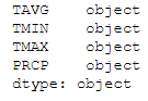I had seen that I had only float64 objects in df_TEMP_PRCP at the start so the problem should have been in df_hds_TEMP_PRCP. Indeed, there the temperatures were objects and not float64 and when I tried to convert them got this error message: Ok, that was unexpected. There were some dashes in the data in some columns and I didn't find them as they are not considered na. I located these rows. 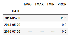Then checked in the first dataset, if I have any values for them. 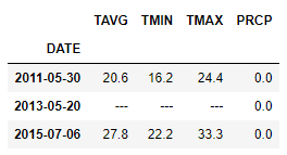I had in the two of the three rows, so here I choose to drop them and move on with my analysis.

df_hds_TEMP_PRCP[(df_hds_TEMP_PRCP.TMIN == '---') | (df_hds_TEMP_PRCP.TMAX == '---') | (df_hds_TEMP_PRCP.TAVG == '---')].index

DatetimeIndex(['2011-05-30', '2013-05-20', '2015-07-06'], dtype='datetime64[ns]', name='DATE', freq=None)

convert_dict = {'TMIN': float,
                'TMAX': float,
                'TAVG': float
               }

df_hds_TEMP_PRCP.drop(labels=[pd.Timestamp('2011-05-30 00:00:00'), pd.Timestamp('2013-05-20 00:00:00'), pd.Timestamp('2015-07-06 00:00:00')], inplace=True)

df_hds_TEMP_PRCP = df_hds_TEMP_PRCP.astype(convert_dict)

df_hds_TEMP_PRCP.dtypes

TAVG    float64
TMAX    float64
TMIN    float64
PRCP    float64
dtype: object

We now fill the na values of the df_TEMP_PRCP dataframe with the values from the df_hds_TEMP_PRCP dataframe.

df_TEMP_PRCP.fillna(df_hds_TEMP_PRCP, inplace=True)

df_TEMP_PRCP[(df_TEMP_PRCP.index.year>=2010) & (df_TEMP_PRCP.index.year<2020)]

	TAVG	TMIN	TMAX	PRCP
DATE
2010-01-01	18.0	17.8	21.8	0.2
2010-01-02	16.0	13.8	17.8	0.0
2010-01-03	13.5	10.8	15.6	0.0
2010-01-04	8.9	5.8	11.0	0.0
2010-01-05	13.1	8.6	16.0	0.0
...	...	...	...	...
2019-12-27	9.8	6.2	13.4	0.0
2019-12-28	8.6	8.2	10.8	0.0
2019-12-29	5.9	3.8	8.0	17.5
2019-12-30	4.2	3.9	7.7	4.6
2019-12-31	5.9	2.8	6.5	37.6

2799 rows × 4 columns

Perfect, now the data in the columns of df_TEMP_PRCP are filled and we have everything we need... Well, that is almost the case. Notice though that there 2799 rows in the dataframe instead of 3649 that should have been there (noticed this in the number of rows of the df_hds dataframe). So, let's go on and fill these rows as well. To do this, we find the difference in indexes between the two dataframes and then we concatenate them.

index_difference = df_hds_TEMP_PRCP.index.difference(df_TEMP_PRCP.index)

len(index_difference)

852

The length of the difference is 852 as expected but it's nice when we take the time to confirm things.

df_TEMP_PRCP = pd.concat([df_TEMP_PRCP, df_hds_TEMP_PRCP.loc[index_difference]], axis=0).sort_index()

df_TEMP_PRCP[(df_TEMP_PRCP.index.year>=2010) & (df_TEMP_PRCP.index.year<2020)].shape

(3651, 4)

df_TEMP_PRCP[(df_TEMP_PRCP.index.year>=2010) & (df_TEMP_PRCP.index.year<2020)].isna().sum()

TAVG    0
TMIN    0
TMAX    0
PRCP    0
dtype: int64

For now, it seems ok and we don't need the second dataframe anymore.

As a sidenote, I noticed that there were discrepancies in the values of the second dataset to the values of the first. For our analysis, I choose to keep the values of the first set and only fill missing values from the second. I could take their average or keep the values from the second dataset, but I choose not to as the purpose of our initial research was only to fill missing values.

Let's check the dataframe now.

df_TEMP_PRCP.isna().sum()

TAVG    2311
TMIN     338
TMAX      83
PRCP     348
dtype: int64

There are still missing values. We will try to cover the TAVG by taking the average of TMIN and TMAX. This, of course, is not totally correct as in a day we could have values near TMIN or TMAX for most of the day so the average isn't accurate but just to have an estimation and better fill our data.

df_TEMP_PRCP.TAVG = df_TEMP_PRCP.TAVG.fillna((df_TEMP_PRCP.TMIN + df_TEMP_PRCP.TMAX)/2)

df_TEMP_PRCP.dtypes

TAVG    float64
TMIN    float64
TMAX    float64
PRCP    float64
dtype: object

df_TEMP_PRCP.isna().sum()

TAVG      1
TMIN    338
TMAX     83
PRCP    348
dtype: int64

df_TEMP_PRCP[df_TEMP_PRCP.TAVG.isna()]

	TAVG	TMIN	TMAX	PRCP
DATE
1957-03-09	NaN	NaN	16.9	0.3

Q2: Deviation of Summer Temperatures

The Hellenic National Meteorological Service has published a report on extreme weather events for 2020. The report is available at http://www.hnms.gr/emy/en/pdf/2020_GRsignificantEVENT_en.pdf. In page 7 of the report there is a graph showing the mean summer temperature deviation from a baseline of 1971-2000.

We will try to create our own version of the graph, using a baseline of 1974-1999. The graph should look like the one below. The line that runs through the graph is the 10 years rolling average of the deviation from the mean. How can we intepret this figure?

We need to calculate the baseline mean temperature for the summers of 1974-1999. So, let's get the mean summer temperatures of these years.

baseline_mean_temp = df_TEMP_PRCP[(df_TEMP_PRCP.index.year>=1974) & (df_TEMP_PRCP.index.year<=1999) & (df_TEMP_PRCP.index.month>=6) & (df_TEMP_PRCP.index.month<=8)].TAVG.mean()

df_TEMP_PRCP_summer = df_TEMP_PRCP[(df_TEMP_PRCP.index.month>=6) & (df_TEMP_PRCP.index.month<=8)]

df_summer_means = df_TEMP_PRCP_summer['TAVG'].groupby(df_TEMP_PRCP_summer.index.year).mean()

df_summer_means_dif = df_summer_means - baseline_mean_temp

df_summer_means_dif

DATE
1955   -0.279640
1956    0.912751
1957    1.141012
1958    0.850794
1959    0.170360
          ...   
2015    1.092099
2016    1.923620
2017    1.857316
2018    1.206229
2019    1.804055
Name: TAVG, Length: 65, dtype: float64

df_rolling = df_summer_means_dif.rolling(window=10, min_periods=1).mean()

from IPython.core.display import HTML
HTML("""
<style>
.output_png {
    display: table-cell;
    text-align: center;
    vertical-align: middle;
}
</style>
""")

fig, ax = plt.subplots(nrows=1, ncols=1, figsize=(12,12))
ax.set_axisbelow(True)
plt.rcParams.update({'axes.titlesize': 'x-large'})
ax.set_title('Mean Summer Temperature Difference from the 1974-1999 Mean', {'fontsize': plt.rcParams['axes.titlesize']})
ax.spines['top'].set_visible(False)
ax.spines['right'].set_visible(False)
ax.spines['bottom'].set_visible(False)
ax.spines['left'].set_visible(False)
colors = ['#FF8C00' if i>0 else "#1111FD" for i in df_summer_means_dif]
plt.bar(df_summer_means_dif.index, df_summer_means_dif, width=0.2, color=colors)
ax.set_facecolor('#E5E5E5')
plt.grid(color='w')
plt.plot([1955, 2019], [0, 0], color='#777777')
plt.plot(df_rolling.index, df_rolling, color='#B5A3DB')

[<matplotlib.lines.Line2D at 0x27d99b8e500>]

The figure shows us that years from 1956 to 1968 we hotter than the average, then there were two and a half decades of colder than the average summers and in the last almost 30 years there is a steady rise of the mean summers temperature, something that is really alarming and concides with the warnings scientists give about global warming.

Q3: Evolution of Daily Temperatures

Now, we will get the average temperate for each year for the full period from 1955 to 2020. We then create a plot showing the daily temperature for each year. The line corresponding to each year will be smoothed by using a 30 days rolling average. The lines are colored from light orange to dark orange, progressing through the years in ascending order.

On that plot we overlay a line showing the average daily temperature for the baseline period of 1974-1999 (that is the black line). The line will also be smoothed usng a 30 years rolling average. How can we interpret this figure?

df_TEMP_PRCP.index.date

array([datetime.date(1955, 1, 1), datetime.date(1955, 1, 2),
       datetime.date(1955, 1, 3), ..., datetime.date(2019, 12, 29),
       datetime.date(2019, 12, 30), datetime.date(2019, 12, 31)],
      dtype=object)

Here we set the index as year and day of year and then unstack the series object in order to keep only year as index and have the days as columns.

df_TEMP = df_TEMP_PRCP.set_index([df_TEMP_PRCP.index.year, df_TEMP_PRCP.index.dayofyear]).TAVG

df_TEMP.index.rename(['year', 'dayOfYear'], inplace=True)

df_TEMP = df_TEMP.unstack()

df_TEMP

dayOfYear	1	2	3	4	5	6	7	8	9	10	...	357	358	359	360	361	362	363	364	365	366
year
1955	14.35	10.70	12.70	13.05	13.15	14.25	13.30	15.80	14.7	13.2	...	14.85	14.25	12.0	11.60	10.2	8.55	8.9	9.25	13.80	NaN
1956	16.35	14.50	12.15	11.65	8.60	7.15	9.15	10.35	10.3	8.7	...	11.00	9.80	14.3	12.40	10.3	11.20	8.3	9.00	9.15	8.15
1957	9.80	10.30	10.40	8.10	8.90	8.55	9.65	8.60	7.4	9.5	...	8.90	9.90	9.3	10.20	10.2	9.80	11.9	15.70	15.80	NaN
1958	12.10	11.80	12.10	10.30	8.50	10.20	13.60	15.60	7.8	5.8	...	16.80	16.40	15.3	12.90	13.6	12.40	13.5	11.20	9.00	NaN
1959	10.90	12.45	13.70	15.50	12.55	8.20	7.15	9.40	13.5	12.5	...	12.30	11.85	13.0	12.15	11.8	13.55	13.6	10.50	10.35	NaN
...	...	...	...	...	...	...	...	...	...	...	...	...	...	...	...	...	...	...	...	...	...
2015	4.40	4.50	5.50	11.10	6.20	3.30	3.40	4.20	6.8	13.3	...	13.00	12.60	13.0	12.50	12.4	11.80	12.4	9.90	3.40	NaN
2016	3.80	7.90	11.50	13.40	17.20	16.40	14.10	13.40	13.2	13.2	...	6.80	7.90	9.2	9.10	11.2	10.80	7.2	3.90	3.60	3.40
2017	6.00	8.40	11.10	11.80	13.20	10.60	2.30	0.50	0.8	2.5	...	6.50	7.90	10.6	11.30	12.9	14.30	12.7	11.30	9.70	NaN
2018	11.30	13.70	11.50	9.60	10.40	11.60	13.90	15.20	14.0	13.2	...	13.50	12.50	9.6	6.00	6.9	8.80	10.8	10.60	9.70	NaN
2019	8.30	7.40	6.40	5.70	3.90	4.80	4.40	2.20	8.6	13.3	...	14.50	12.70	11.3	10.60	9.8	8.60	5.9	4.20	5.90	NaN

65 rows × 366 columns

Next, we calculate the rolling average with a window of 30 days.

df_TEMP_rolling = df_TEMP.rolling(window=30).mean()

fig, ax = plt.subplots(nrows=1, ncols=1, figsize=(16,6))
ax.set_axisbelow(True)
ax.set_ylabel('Aberage Daily Temperature')
ax.set_xlabel('Date')
ax.spines['top'].set_visible(False)
ax.spines['right'].set_visible(False)
ax.spines['bottom'].set_visible(False)
ax.spines['left'].set_visible(False)
ax.set_facecolor('#E5E5E5')
plt.grid(color='w')

# got this code snippet from StackOverflow. It maps the days of the year to the appropriate months

import datetime as dt
import matplotlib.dates as mdates
start = dt.datetime(2016,1,1)    #there has to be a year given, even if it isn't plotted
new_dates = [start + dt.timedelta(days=i) for i in range(366)]
x = new_dates
y = df_TEMP.index

xfmt = mdates.DateFormatter('%b')
months = mdates.MonthLocator()
ax.xaxis.set_major_locator(months)
ax.xaxis.set_major_formatter(xfmt)


# Now we plot our lines usings a loop to get the rows one by one
for _, year in df_TEMP_rolling.iterrows():
    plt.plot(year.index, year.values)
    
    

The interpretation of the figure is that the weather is hotter in the summer months and we also notice that darker orange lines are higher. That means that the recent years have been hotter on average than past years.

Q4: Extreme Temperature Events

Another measure used by climatologists is the number of extreme events. Extreme events are defined as those beyond 5% or 10% from the expected value. We will deal with extreme heat events going 10% above the baseline.

We will count the number of extreme temperature events per year, compared to the baseline of 1974-1999. We should be able to produce a graph like the one that follows. The vertical axis is the percentage of extreme heat events calculated over the number of observations for each year. The gray line in the middle is the average percentage of extreme tempearture events of the baseline. The colour blue is used for those years where the percentage is below the baseline; otherwise the colour is orange. How can we interpret this graph?

We calculate the baseline of the temperatures from 1974-1999.

baseline = df_TEMP_PRCP[(df_TEMP_PRCP.index.year>=1974) & (df_TEMP_PRCP.index.year<=1999)].TAVG.mean()

baseline

17.852632687447347

Here we get the days with temperatures above the 110% of the baseline and then we count them.

df_extreme = df_TEMP_PRCP[df_TEMP_PRCP.TAVG > 1.1 * baseline]

df_extreme_days = df_extreme.groupby(df_extreme.index.year).count()

df_extreme_days['years'] = df_extreme_days.index

Calculate number of extreme days between 1974 and 1999.

number_of_extreme_days_74_99 = df_extreme_days[(df_extreme_days.index>=1974) & (df_extreme_days.index<=1999)].TAVG.sum()

# importing calendat to get leap years
import calendar

df_extreme_days['number_of_days_in_year'] = df_extreme_days.years.apply(lambda x: 366 if calendar.isleap(x) else 365)

df_extreme_days['percentage'] = df_extreme_days.TAVG / df_extreme_days.number_of_days_in_year

number_of_baseline_days = df_extreme_days[(df_extreme_days.index>=1974) & (df_extreme_days.index<=1999)]['number_of_days_in_year'].sum()

Calculate baseline percentage.

baseline_percentage = number_of_extreme_days_74_99 / number_of_baseline_days

baseline_percentage

0.413647851727043

fig, ax = plt.subplots(nrows=1, ncols=1, figsize=(12,10))
ax.set_axisbelow(True)
ax.spines['top'].set_visible(False)
ax.spines['right'].set_visible(False)
ax.spines['bottom'].set_visible(False)
ax.spines['left'].set_visible(False)
ax.set_facecolor('#E5E5E5')
plt.grid(color='w')
colors = ['#FF8C00' if i>baseline_percentage else "b" for i in df_extreme_days.percentage]
plt.bar(df_extreme_days.index, df_extreme_days.percentage, width=0.2,color=colors)
plt.axhline(y=baseline_percentage, color='#777777')

<matplotlib.lines.Line2D at 0x23feb68aef0>

The interpretation of the graph is that in recent years extreme heat events are much more prevalent than in the past.

Q5: Precipitation

Continuing the thread on extreme events, another consideration is rainfall. The weather may or may not be drying up. We are, however, interested in whether precipication becomes more intense over time.

To see that, we will count the overall rainfall over the year and the number of rainy days in each year. Then, by dividing the rainfall by the number of rainy days we will get an indication of whether we are getting rain in more concentrated bursts. We will then create a plot showing the ratio of rainfall over rainy days over the years. On the plot we will overlay the 10 years rolling average. The plot should be similar to the one below. How can we interpret this plot?

Firstly, we get the sum of the precipitation for each year.

prcp_sum = df_TEMP_PRCP.groupby(df_TEMP_PRCP.index.year).sum()['PRCP']

Then we make a dataframe with only the days that had some rainfall and count how mnay those days were per year.

df_PRCP = df_TEMP_PRCP[df_TEMP_PRCP.PRCP > 0]

df_PRCP.groupby(df_PRCP.index.year).count()

	TAVG	TMIN	TMAX	PRCP
DATE
1955	68	68	68	68
1956	52	52	52	52
1957	72	72	73	73
1958	68	68	68	68
1959	62	62	62	62
...	...	...	...	...
2015	41	41	41	41
2016	42	42	42	42
2017	48	48	48	48
2018	55	55	55	55
2019	58	58	58	58

65 rows × 4 columns

prcp_num_days = df_TEMP_PRCP[df_TEMP_PRCP.PRCP > 0].groupby(df_TEMP_PRCP[df_TEMP_PRCP.PRCP > 0].index.year).count()['PRCP']

We divide the sum of the rainfall amount in mm of every year with the number that it rained in every year.

prcp_burst = prcp_sum / prcp_num_days

prcp_burst.index

Int64Index([1955, 1956, 1957, 1958, 1959, 1960, 1961, 1962, 1963, 1964, 1965,
            1966, 1967, 1968, 1969, 1970, 1971, 1972, 1973, 1974, 1975, 1976,
            1977, 1978, 1979, 1980, 1981, 1982, 1983, 1984, 1985, 1986, 1987,
            1988, 1989, 1990, 1991, 1992, 1993, 1994, 1995, 1996, 1997, 1998,
            1999, 2000, 2001, 2002, 2003, 2004, 2005, 2006, 2007, 2008, 2009,
            2010, 2011, 2012, 2013, 2014, 2015, 2016, 2017, 2018, 2019],
           dtype='int64', name='DATE')

We calculate the rolling average.

prcp_rolling = prcp_burst.rolling(window=10, min_periods=1).mean()

fig, ax = plt.subplots(nrows=1, ncols=1, figsize=(12,10))
ax.set_axisbelow(True)
ax.spines['top'].set_visible(False)
ax.spines['right'].set_visible(False)
ax.spines['bottom'].set_visible(False)
ax.spines['left'].set_visible(False)
ax.set_facecolor('#E5E5E5')
plt.grid(color='w')
plt.bar(prcp_burst.index, prcp_burst,width=0.3, color='b')
plt.plot(prcp_rolling.index, prcp_rolling)

[<matplotlib.lines.Line2D at 0x23feeb00220>]

My interpretation of the graph is that there is some steady increase in the intensity of the rainfall as we go from the 60's to today.

Parting thoughts

I see that my graphs have a lot of differences to the given graphs. I believe this has to do with the hypothesis that I did early in the study that I can create many average temperatures by averaging min and max temperatures per day. Many of these temperatures created could be way off and play significant role in how the graphs are produced. Maybe it could be safe to leave them as NaN and just have some missing lines in the graphs as the ones depicted.

---

Next Post →

---

Copyright © Christodoulos Santorinaios 2022